Challenge overview
Wiretrace is a Side Channel Attack (SCA) challenge created by Neige for FCSC 2026. It was released as a three ⭐ difficulty challenge (the highest diffculty) and was solved by three players.
The challenge name is a play on words for Wire Trace / Weierstrass which works quite well when pronounced with a bad French accent.
For this challenge we are given two files:
- “Protocole_de_communication.md” is a Markdown file with some documentation about the communication protocol used between the CPU and the hardware accelerator.
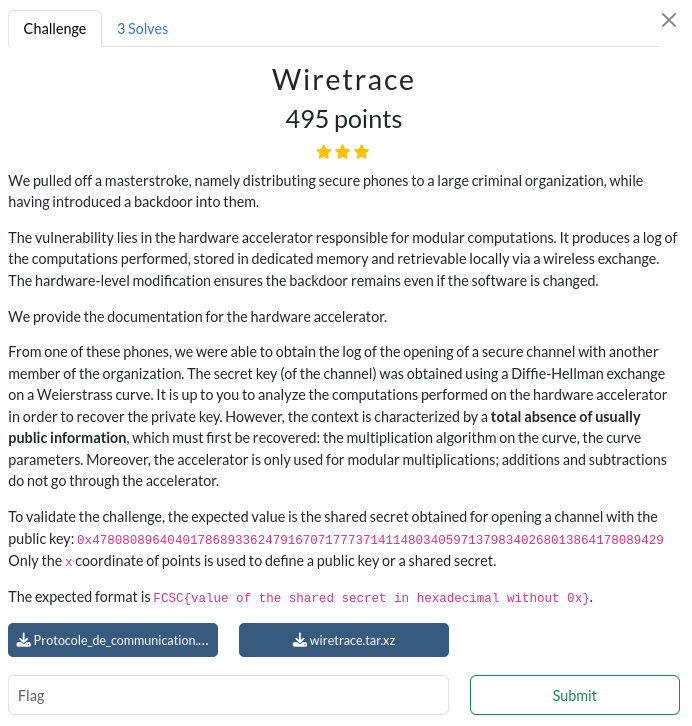
- “wiretrace” is a sigrok text export of a logic capture (libsigrok 0.5.1, Acquisition with 8/12 channels at 500 MHz). From this capture we should be able to find the modular operations that were executed by the hardware accelerator.
From the challenge description, the trace should contain logs of modular operations executed during a Diffie-Hellman exchange on a Weierstrass curve (aka ECDH / Elliptic Curve Diffie-Hellman). The goal is to analyze the logs in order to recover the private key used during the exchange, and then use it to compute a new shared secret.
- Link to challenge files: TODO - will be available on https://hackropole.fr soon.
Wiretrace file format
First we need to understand the format of the “wiretrace” file.
libsigrok 0.5.1
Acquisition with 8/12 channels at 500 MHz
D0:00001111 11101011 10011111 10011111 11111111 10000000 00000000 00000000
D1:00100011 11100111 11100111 00011111 00111111 10000000 00000000 00000000
D2:01101001 11101111 10000111 10001111 11011111 11000000 00000000 00000000
D3:01001111 11100111 10001111 10011111 10011111 10000000 00000000 00000000
D4:00001111 10011111 11011111 10101111 10111111 11000000 00000000 00000000
D5:01111111 10010011 10101111 10001111 11111111 11000000 00000000 00000000
D6:10111011 11101111 10000111 11101111 10011111 10000000 00000000 00000000
D7:11000111 11101111 10000111 11111111 11111111 11000000 00000000 00000000
D0:00000000 00000000 00000000 00000000 00000000 10000000 00000101 01011000
D1:00000000 00000000 00000000 00000000 00000000 10000000 00001001 11011011
D2:00000000 00000000 00000000 00000000 00000001 10000000 01011011 10101000
D3:00000000 00000000 00000000 00000000 00000001 00000000 01001110 01101000
D4:00000000 00000000 00000000 00000000 00000000 10000000 00001010 10111111
D5:00000000 00000000 00000000 00000000 00000001 10000000 01010011 10111100
D6:00000000 00000000 00000000 00000000 00000010 10000000 00101000 00000000
D7:00000000 00000000 00000000 00000000 00000011 00000000 01100100 00101110
D0:00000010 01000000 10010001 00100000 00000000 00101010 11000000 00010010
[...]
D0:10000111 10000001 00110110 11100000 00
D1:00000100 00110111 01011011 01100000 00
D2:11110001 10010111 10101100 00100000 00
D3:11011001 00000111 01000011 10100000 00
D4:11011010 10111101 10011110 11100000 00
D5:01000001 00010111 11111010 01000000 00
D6:01111001 10000101 11000111 10100000 00
D7:01100000 00110101 01111110 11000000 00
The first line is just a header, the second line indicates an acquisition of 8 distinct channels at 500 MHz, and the remaining lines are the bit values sampled during that acquisition. The text file is not too difficult to parse. I decided to export the first few samples of each channel to a CSV file, so that I could open it with pulseview and visualize the signal over time.
bits_per_channel = [[] for _ in range(8)]
with open('wiretrace', 'r') as f:
    for line in f:
        line = line.strip()
        if not line.startswith('D'):
            continue
        Di, bits = line.strip().split(':')
        channel = int(Di[1])
        bits_per_channel[channel].extend(b for b in bits if b in '01')

with open('wiretrace.csv', 'w') as f:
    f.write('D0,D1,D2,D3,D4,D5,D6,D7\n')
    for i in range(1000):
        f.write(','.join(bits[i] for bits in bits_per_channel) + '\n')
Opening the CSV file with pulseview yields a very satisfying visualization. The 8 channels look synchronized and there does not seem to be a clock signal or a complicated serial communication protocol. It is actually a simple 8-bit parallel synchronous bus and can be decoded with the “Parallel sync bus (parallel)” decoder with default parameters.
Zooming in on the protocol decoder output confirms that the decoding is correct. The result matches the communication protocol documentation. For example the image below corresponds to two frames.
- “c0 | ac | 77” maps to “| senderId | receiverId | opcode |”, where 0x77 is the opcode for “Demande de réponse”, sent to the hardware accelerator.
- “ac | c0 | 001ab26078f3…” maps to “| senderId | receiverId | operand1 |”, where 0x001ab26078f3… is the result of the previous operation, sent by the hardware accelerator.

Communication frames extraction
Now we can parse the original file again, convert to raw bytes, and extract all the messages exchanged between the ECC block and the modular accelerator. After some trial and error we also find some additional useful information.
- The trace only contains opcodes 0x55 (modular multiplication request), 0x66 (modular square request), 0x77 (request for the result of the operation), and the results sent by the accelerator.
- The parameter “t” (the byte length of operands and results) is 40.
- All operands seem to be encoded in big-endian format (the value “0x1” is more likely than 0x1000000000000000000000000000000000000000000000000000000000000000000000000000000).
import os

# Convert parallel bus data to raw bytes
if not os.path.exists('wiretrace.raw'):
    # Extract bits
    bits_per_channel = [[] for _ in range(8)]
    with open('wiretrace', 'r') as f:
        for line in f:
            line = line.strip()
            if not line.startswith('D'):
                continue
            Di, bits = line.strip().split(':')
            channel = int(Di[1])
            bits_per_channel[channel].extend(b for b in bits if b in '01')
    # Convert to raw bytes
    L = len(bits_per_channel[0])
    data = [int(''.join(bits_per_channel[i][j] for i in range(7,-1,-1)), 2) for j in range(L)]
    with open('wiretrace.raw', 'wb') as f:
        f.write(bytes(data))
    exit()
with open('wiretrace.raw', 'rb') as f:
    data = f.read()
L = len(data)

# Parse protocol messages
ECC_ID   = 0xc0
ACCEL_ID = 0xac
T        = 40
REQUEST = None
i = 0
while i < L:
    sender, receiver = data[i], data[i+1]
    assert sender != receiver and sender in [ECC_ID, ACCEL_ID] and receiver in [ECC_ID, ACCEL_ID]
    i += 2
    if sender == ECC_ID:
        opcode = data[i]
        i += 1
        if opcode == 0x55: # Modular multiplication request
            op1 = int.from_bytes(data[i:i+T])
            op2 = int.from_bytes(data[i+T:i+T+T])
            REQUEST = ('MULTIPLY', op1, op2)
            print(f'MULTIPLY {op1:x} {op2:x}')
            i += 2 * T
        elif opcode == 0x66: # Modular square request
            op1 = int.from_bytes(data[i:i+T])
            REQUEST = ('SQUARE', op1)
            print(f'SQUARE   {op1:x}')
            i += T
        elif opcode == 0x77: # Request for the result
            pass
        else:
            assert False, f'Unknown opcode {hex(opcode)}'
        pass
    else:
        # Result
        assert REQUEST is not None
        result = int.from_bytes(data[i:i+T])
        REQUEST = None
        print(f'RESULT   {result:x}')
        print()
        i += T
    # Skip null bytes between messages
    while i < L and data[i] == 0:
        i += 1
The first few messages are successive squaring operations, showing a nice decreasing pattern. After that, all remaining values found in the trace are less than $2^{255}$.
SQUARE   607db9fbffffcfcf30d5deffffff12221139fffffffdc0d08bfffffffffda5b3ffffffffffffb400
RESULT   245e893c27360bbc33bfb092122eeebe9264a489f8bc67d2c670144c1c8d4072899a4ec06164bc37

SQUARE   245e893c27360bbc33bfb092122eeebe9264a489f8bc67d2c670144c1c8d4072899a4ec06164bc37
RESULT   52ab981fcc56f17f1599ec65969032c6cd9cb2a400df73e0f1915f703d8e555d4e155a06d599ca5

SQUARE   52ab981fcc56f17f1599ec65969032c6cd9cb2a400df73e0f1915f703d8e555d4e155a06d599ca5
RESULT   1ab26078f3c875890c75a4f29b41bcfbde0a8681526e6803fabd1b85eb566569864c9624c8777d

SQUARE   1ab26078f3c875890c75a4f29b41bcfbde0a8681526e6803fabd1b85eb566569864c9624c8777d
RESULT   2c8b7e2de12c5e9996838ed174d6ac96cfde2ac5f8197ba732c9da51f2c048d296a1179e85c

SQUARE   2c8b7e2de12c5e9996838ed174d6ac96cfde2ac5f8197ba732c9da51f2c048d296a1179e85c
RESULT   7c03f6d7e0fd7668bd1799d9f663b6561de25d7d2502818dd7dfa3e332383f7d2cfcc

SQUARE   7c03f6d7e0fd7668bd1799d9f663b6561de25d7d2502818dd7dfa3e332383f7d2cfcc
RESULT   17cf6e6545d2720f9543ce9d03f46b48323dff745e90331e55e1bd6191ba0424

MULTIPLY 17cf6e6545d2720f9543ce9d03f46b48323dff745e90331e55e1bd6191ba0424 1
RESULT   219a266e262f8716d482aebb63a22ac61575502814c37e5cf3332383f3dbaac5

MULTIPLY 219a266e262f8716d482aebb63a22ac61575502814c37e5cf3332383f3dbaac5 1
RESULT   128a91347d05f46cb119f52b9a3df6b7ce6c2a12e9a7e0db7ba8a33509ff2c04

MULTIPLY 2523648240000001ba344d80000000086121000000000013a700000000000012 219a266e262f8716d482aebb63a22ac61575502814c37e5cf3332383f3dbaac5
RESULT   1298d34dc2fa0b95091a585465c2095092b4d5ed16581f382b575ccaf600d40f

MULTIPLY 1 219a266e262f8716d482aebb63a22ac61575502814c37e5cf3332383f3dbaac5
RESULT   128a91347d05f46cb119f52b9a3df6b7ce6c2a12e9a7e0db7ba8a33509ff2c04

MULTIPLY 25152268fa0be8d96233ea57347bed6f9cd85425d34fc1b6f751466a13fe5808 128a91347d05f46cb119f52b9a3df6b7ce6c2a12e9a7e0db7ba8a33509ff2c04
RESULT   25152268fa0be8d96233ea57347bed6f9cd85425d34fc1b6f751466a13fe5808

SQUARE   1298d34dc2fa0b95091a585465c2095092b4d5ed16581f382b575ccaf600d40f
RESULT   128a91347d05f46cb119f52b9a3df6b7ce6c2a12e9a7e0db7ba8a33509ff2c04

MULTIPLY 25152268fa0be8d96233ea57347bed6f9cd85425d34fc1b6f751466a13fe5808 128a91347d05f46cb119f52b9a3df6b7ce6c2a12e9a7e0db7ba8a33509ff2c04
RESULT   25152268fa0be8d96233ea57347bed6f9cd85425d34fc1b6f751466a13fe5808

MULTIPLY 4a2a44d1f417d1b2c467d4ae68f7dadf39b0a84ba69f836deea28cd427fcb010 1298d34dc2fa0b95091a585465c2095092b4d5ed16581f382b575ccaf600d40f
RESULT   1c84328be82e50b000c65197082531889157b459607cb95f5d732bd8035016

MULTIPLY 25152268fa0be8d96233ea57347bed6f9cd85425d34fc1b6f751466a13fe5808 4a2a44d1f417d1b2c467d4ae68f7dadf39b0a84ba69f836deea28cd427fcb010
RESULT   24ea5c1d282fa3605a32c0dcd1efb5a54ffe50974d3f06a0e84519a84ff95fe7
Montgomery form / Montgomery multiplication
The first two MULTIPLY operations are very troubling. It seems that the hardware accelerator computed 0x17cf... * 0x1 = 0x219a... and 0x219a... * 0x1 = 0x128a..., which does not make much sense.
MULTIPLY 17cf6e6545d2720f9543ce9d03f46b48323dff745e90331e55e1bd6191ba0424 1
RESULT   219a266e262f8716d482aebb63a22ac61575502814c37e5cf3332383f3dbaac5

MULTIPLY 219a266e262f8716d482aebb63a22ac61575502814c37e5cf3332383f3dbaac5 1
RESULT   128a91347d05f46cb119f52b9a3df6b7ce6c2a12e9a7e0db7ba8a33509ff2c04
Similarly, a few lines below, we find the operation 0x2515... * 0x128a... = 0x2515... (a * b = a).
MULTIPLY 25152268fa0be8d96233ea57347bed6f9cd85425d34fc1b6f751466a13fe5808 128a91347d05f46cb119f52b9a3df6b7ce6c2a12e9a7e0db7ba8a33509ff2c04
RESULT   25152268fa0be8d96233ea57347bed6f9cd85425d34fc1b6f751466a13fe5808
This does not make any sense when working with ordinary modular multiplications, whatever the modulus could be.
I got stuck at this point for some time, until I remembered that the FCSC virtual machine used for assembly programming challenges, as well as other Side Channel / Fault injection challenges, also implements a “hardware accelerator”.
- https://fcsc.fr/vm___g1iJVwC3NFka5dowCrhDMhUUvgUCYLta___ - FCSC virtual machine documentation.
More specifically, it implements Montgomery modular multiplication, a method for performing fast modular multiplication which avoids expensive division operations.
Montgomery Multiplication    MM Ro, Rm, Rn    -    Ro = Rm*Rn/R mod FPmodule
Montgomery Multiplication    MM1 Rj, Ri       -    Rj = Ri/R mod FPmodule
Montgomery Exponentiation    MPOW Rj, Ri      -    Rj = (Ri/R)**RC*R mod FPmodule
Using the classical “residue class” number representation modulo $N$, the modular multiplication of $a$ and $b$ requires computing the quotient $q = \lfloor (a \times b) / N \rfloor$ in order to find the remainder $r = ab - qN$. The computation of $q$ therefore requires a division by $N$, which is usually a very expensive computation on most computer hardware.
Montgomery multiplication instead relies on a special representation of elements of the ring $\mathbb{Z}/N\mathbb{Z}$ , the “Montgomery form”. In this form, modular products only require a division by some fixed divisor $R$, instead of $N$. The value of $R$ can be chosen in advance such that the division is always fast. A good choice of $R$ is a large enough power of two, for which division can be replaced by a simple bit shift / truncation.
Montgomery arithmetic is defined as follows.
- The Montgomery form of the residue class $\overline{a}$ with respect to the divisor $R$ is simply $aR \pmod{N}$.
- Addition and subtraction in Montgomery form is the same as usual modular addition and modular subtraction, $(aR + bR) = (a+b)R$.
- Multiplication in Montgomery form is different. The usual product $(aR)(bR)=(abR)R$ has an extra factor $R$, which must be removed with division by $R$. This can be done by multiplying the result by $R^{-1} \pmod{N}$.
The straightforward way to multiply numbers in Montgomery form is therefore to multiply the integers $aR \pmod{N}$, $bR \pmod{N}$ and $R^{-1} \pmod{N}$ and then reduce the result modulo $N$. This is of course very inefficient because it requires division by $N$ at the end, which is exactly what we are trying to avoid.
Fortunately, the Montgomery Reduction algorithm (aka REDC) is an efficient algorithm that can both compute the product by $R^{-1} \pmod{N}$ and reduce the result modulo $N$, using only reductions and divisions by $R$, not $N$.
In order to compute $(aR)(bR)/R \pmod{N}$, the algorithm finds a small integer $k$ such that $(aRbR)+kN$ is a multiple of $R$. The integer division of $(aRbR)+kN$ by $R$ is fast, and the final reduction modulo $N$ only requires a simple subtraction.
- https://en.wikipedia.org/wiki/Montgomery_modular_multiplication#The_REDC_algorithm - More information about the REDC algorithm.
We can assume that all numbers we found in the trace are in Montgomery form for some integer $R$, and that multiplication is actually Montgomery multiplication. With this hypothesis in mind, we can find the value of $R$ modulo $N$ from the following equation.
MULTIPLY 25152268fa0be8d96233ea57347bed6f9cd85425d34fc1b6f751466a13fe5808 128a91347d05f46cb119f52b9a3df6b7ce6c2a12e9a7e0db7ba8a33509ff2c04
//       a * R                                                            b * R
RESULT   25152268fa0be8d96233ea57347bed6f9cd85425d34fc1b6f751466a13fe5808
//       a * R

=> [(a * R) * (b * R) / R] (mod N) == a * R (mod N)
=> a * b * R == a * R (mod N)
=> b = 1 (mod N)
=> R = 0x128a91347d05f46cb119f52b9a3df6b7ce6c2a12e9a7e0db7ba8a33509ff2c04 (mod N)
Then to find the value of the modulus $N$ I used the next two equations.
MULTIPLY 1             219a266e262f8716d482aebb63a22ac61575502814c37e5cf3332383f3dbaac5
//       R^-1 * R      a * R
RESULT   128a91347d05f46cb119f52b9a3df6b7ce6c2a12e9a7e0db7ba8a33509ff2c04
//       1 * R

=> [(R^-1 * R) * (a * R) / R] (mod N) == 1 * R (mod N)
=> a = R (mod N)
=> (a * R) - R^2 = k1 * N

SQUARE   1298d34dc2fa0b95091a585465c2095092b4d5ed16581f382b575ccaf600d40f
//       b * R
RESULT   128a91347d05f46cb119f52b9a3df6b7ce6c2a12e9a7e0db7ba8a33509ff2c04
//       1 * R

=> [(b * R) * (b * R) / R] (mod N) = 1 * R (mod N)
=> b^2 * R = R (mod N)
=> (b * R)^2 - R^2 = k2 * N
We find the value of $N$ from the two equations by taking a GCD, it turns out to be a 254-bit prime number with a nice hexadecimal representation. At this point we can start calling it $p$.
R  = 0x128a91347d05f46cb119f52b9a3df6b7ce6c2a12e9a7e0db7ba8a33509ff2c04
aR = 0x219a266e262f8716d482aebb63a22ac61575502814c37e5cf3332383f3dbaac5
bR = 0x1298d34dc2fa0b95091a585465c2095092b4d5ed16581f382b575ccaf600d40f
N = gcd(aR - R**2, bR**2 - R**2)
assert N == 0x2523648240000001ba344d80000000086121000000000013a700000000000013
assert is_prime(N)
p = N
assert p.bit_length() == 254
Finding the curve
Now that we know both the modulus $p$ and the Montgomery divisor $R$ (only modulo $p$), we can convert every number in the trace to the usual representation, by multiplying everything by $R^{-1} \pmod{p}$.
from sage.all import GF

# Parse protocol messages and convert everything back from Montgomery form
ECC_ID   = 0xc0
ACCEL_ID = 0xac
T        = 40
p = 0x2523648240000001ba344d80000000086121000000000013a700000000000013
F = GF(p)
R = F(0x128a91347d05f46cb119f52b9a3df6b7ce6c2a12e9a7e0db7ba8a33509ff2c04)
R_inv = R.inverse()
REQUEST = None
OPERATIONS = []
i = 0
while i < L:
    sender, receiver = data[i], data[i+1]
    assert sender != receiver and sender in [ECC_ID, ACCEL_ID] and receiver in [ECC_ID, ACCEL_ID]
    i += 2
    if sender == ECC_ID:
        opcode = data[i]
        i += 1
        if opcode == 0x55: # Modular multiplication request
            op1 = F(int.from_bytes(data[i:i+T])) * R_inv
            op2 = F(int.from_bytes(data[i+T:i+T+T])) * R_inv
            REQUEST = ('MULTIPLY', op1, op2)
            print(f'MULTIPLY {int(op1):x} {int(op2):x}')
            i += 2 * T
        elif opcode == 0x66: # Modular square request
            op1 = F(int.from_bytes(data[i:i+T])) * R_inv
            REQUEST = ('SQUARE', op1)
            print(f'SQUARE   {int(op1):x}')
            i += T
        elif opcode == 0x77: # Request for the result
            pass
        else:
            assert False, f'Unknown opcode {hex(opcode)}'
        pass
    else:
        # Result
        assert REQUEST is not None
        result = F(int.from_bytes(data[i:i+T])) * R_inv
        if REQUEST[0] == 'MULTIPLY':
            assert result == REQUEST[1] * REQUEST[2]
            OPERATIONS.append(('MULTIPLY', REQUEST[1], REQUEST[2]))
        else:
            assert result == REQUEST[1]**2
            OPERATIONS.append(('SQUARE', REQUEST[1]))
        REQUEST = None
        print(f'RESULT   {int(result):x}')
        print()
        i += T
    # Skip null bytes between messages
    while i < L and data[i] == 0:
        i += 1
With the numbers converted back from Montgomery form, the operations now look much nicer and make a lot more sense!
SQUARE   400
RESULT   100000

SQUARE   100000
RESULT   10000000000

SQUARE   10000000000
RESULT   100000000000000000000

SQUARE   100000000000000000000
RESULT   10000000000000000000000000000000000000000

SQUARE   10000000000000000000000000000000000000000
RESULT   128a91347d05f46cb119f52b9a3df6b7ce6c2a12e9a7e0db7ba8a33509ff2c04

SQUARE   128a91347d05f46cb119f52b9a3df6b7ce6c2a12e9a7e0db7ba8a33509ff2c04
RESULT   219a266e262f8716d482aebb63a22ac61575502814c37e5cf3332383f3dbaac5

MULTIPLY 219a266e262f8716d482aebb63a22ac61575502814c37e5cf3332383f3dbaac5 c09b8b2cae1000503213a4d431ac4b50f963e91e154cb9f20b402076b38149
RESULT   128a91347d05f46cb119f52b9a3df6b7ce6c2a12e9a7e0db7ba8a33509ff2c04

MULTIPLY 128a91347d05f46cb119f52b9a3df6b7ce6c2a12e9a7e0db7ba8a33509ff2c04 c09b8b2cae1000503213a4d431ac4b50f963e91e154cb9f20b402076b38149
RESULT   1

MULTIPLY 2462c8f71351f0016a0239db2bce53bd10279c16e1eab359b4f4bfdf894c7eca 128a91347d05f46cb119f52b9a3df6b7ce6c2a12e9a7e0db7ba8a33509ff2c04
RESULT   2523648240000001ba344d80000000086121000000000013a700000000000012

MULTIPLY c09b8b2cae1000503213a4d431ac4b50f963e91e154cb9f20b402076b38149 128a91347d05f46cb119f52b9a3df6b7ce6c2a12e9a7e0db7ba8a33509ff2c04
RESULT   1

MULTIPLY 2 1
RESULT   2

SQUARE   2523648240000001ba344d80000000086121000000000013a700000000000012
RESULT   1

MULTIPLY 2 1
RESULT   2

MULTIPLY 4 2523648240000001ba344d80000000086121000000000013a700000000000012
RESULT   2523648240000001ba344d80000000086121000000000013a70000000000000f

MULTIPLY 2 4
RESULT   8

MULTIPLY 2 2
RESULT   4
The initial square operations are the computation of the divisor $R = 2^{320}= 400_h^{32}$, the clean power of two used by Montgomery multiplication. We can also find the value of $R^{-1}$ (0xc09b8b…) in a few operations. Using Montgomery form, these operations are $R^3 \times 1$, $R^2 \times 1$ and $1 \times R^2$.
After that, we also find multiplication and squaring of small values modulo $p$.
At this point we have enough information to find the curve. If we look up the value of $p$ (0x2523648240000001BA344D80000000086121000000000013A700000000000013), we find that is the modulus used by the curve BN254. The coordinates of the generator point $G=$ (0x2523648240000001BA344D80000000086121000000000013A700000000000012, 0x1) of this curve are also repeatedly found in the trace, which is a good sign.
- https://std.neuromancer.sk/bn/bn254 - More information about the BN254 curve.
The big picture
Before digging into the 9380 individual operations we find in the trace, it’s nice to look at the big picture and see if we can find any pattern in the operations. In the image below, black lines are “SQUARE” operations and white lines “MULTIPLY” (Click here and zoom in to see better).

There is a clear pattern in the trace.
- A very long pattern of interlaced multiplications and squaring.
- A smaller strip of mostly squaring operations.
- Another very long pattern of both multiplications and squaring.
- At the end, a final smaller strip of mostly squaring operations.
The challenge description states that this is the trace of the computation for an ECDH key exchange. Recall how the exchange is supposed to work.
- Let $G$ be the generator point of a pre-defined elliptic curve (here we are using BN254) of order $n$.
- Alice chooses a secret integer $n_A \leq n-1$ and computes the public point $P_A = n_AG$.
- Bob chooses a secret integer $n_B \leq n-1$ and computes the public point $P_B = n_BG$.
- Alice sends $P_A$ to Bob and Bob sends $P_B$ to Alice, over a potentially insecure channel.
- Alice computes $n_AP_B$ and Bob computes $n_BP_A$.
- The shared secret between Alice and Bob is $n_AP_B=n_BP_A=n_An_BG$.
The only two operations for Alice are the computation of $n_A G$ and $n_A P_B$. There are multiple algorithms for elliptic curve scalar multiplication (adding a point to itself repeatedly), but they all require computing a large number of point addition and point doubling operations, which themselves require the computation of multiple modular operations.
Most likely the two large blocks in the trace are the computation of $n_AG$ and $n_A P_B$. Now we can start to see the path to the solution.
- From the MULTIPLY / SQUARE operations patterns, identify the “point addition” and “point doubling” operations.
- From the point doubling and point addition operations, identify the elliptic curve scalar multiplication algorithm that is used.
- From the knowledge of the scalar multiplication algorithm and the point doubling / addition operations, recover the bits of the secret integer $n_A$.
So the next thing we need to do is to identify whether a block of successive modular operations corresponds to point addition or point doubling. This is actually easy to do by simply checking if the point coordinates of $G$ appear in the operations (in which case we are looking at point addition with $G$), or not (then it’s point doubling).
Point addition / point doubling formulas
This section is completely overkill to solve the challenge. It was absolutely NOT REQUIRED to identify the exact formula used for point addition and point doubling. All we need is to distinguish between them and it is not hard to do. I decided to do it anyway because I was starting to doubt a lot of things (possibly because I didn’t read half of the challenge description).
At first I tried to find the coordinates of the point $2G$ in the trace.
sage: p = 0x2523648240000001BA344D80000000086121000000000013A700000000000013
....: K = GF(p)
....: a = K(0x0000000000000000000000000000000000000000000000000000000000000000)
....: b = K(0x0000000000000000000000000000000000000000000000000000000000000002)
....: E = EllipticCurve(K, (a, b))
....: G = E(0x2523648240000001BA344D80000000086121000000000013A700000000000012, 0x0000000000000000000000000000000000000000000000000000000000000001)
....: E.set_order(0x2523648240000001BA344D8000000007FF9F800000000010A10000000000000D * 0x01)
sage: hex((2 * G).x())
'0x948d920900000006e8d1360000000021848400000000004e9c0000000000009'
Unfortunately the value of the $x$ coordinate, 0x948d920900000006e8d1360000000021848400000000004e9c0000000000009, is nowhere to be found in the list of modular operations, which was very concerning. But if we think about it a little more, it actually makes sense.
Most efficient implementations do not use affine coordinates $(x, y)$ to represent points, but instead projective coordinates $(X, Y, Z)$. More specifically, a common representation for elliptic curves in short Weierstrass form ($y^2+xy=x^3+a_2x^2+a_6$) is known as Jacobian coordinates, with $x=X/Z^2$ and $y= Y/Z^3$.
There are many explicit formulas for point addition / doubling in Jacobian coordinates. They have different modular operation counts (“costs”) and some can only be used under certain assumptions. After spending some time computing a list of intermediate values used by some of these formulas, I managed to find the ones used in this challenge (or close enough). This was made harder by the fact that the trace only contains multiplication and squaring operations, missing modular addition and subtraction.
Fortunately the formulas used here are common enough to be found at the top of the list at https://www.hyperelliptic.org/EFD/g12o/auto-shortw-jacobian.html. In the following example, we find the computation of $2P$ with $P=(X_1,Y_1,Z_1)=$ (0x11, 0x2523648240000001ba344d80000000086121000000000013a6ffffffffffffcc, 0x2) using what I identified as the “dbl-2009-l” formula: https://www.hyperelliptic.org/EFD/g1p/auto-shortw-jacobian-0.html#:~:text=dbl-2009-l.
(X, Y, Z) = (0x11, 0x2523648240000001ba344d80000000086121000000000013a6ffffffffffffcc, 0x2)

# 2 * Y1 = Y1 + Y1 = 0x2523648240000001ba344d80000000086121000000000013a6ffffffffffff85
# (2 * Y1) * Y1 = 2 * B <-- part of D computation
MULTIPLY 2523648240000001ba344d80000000086121000000000013a6ffffffffffff85 2523648240000001ba344d80000000086121000000000013a6ffffffffffffcc
RESULT   2762

# A = X1 * X1
SQUARE   11
RESULT   121

# Z3 = (2 * Y1) * Z1
MULTIPLY 2523648240000001ba344d80000000086121000000000013a6ffffffffffff85 2
RESULT   2523648240000001ba344d80000000086121000000000013a6fffffffffffef7

# (4 * B) * X1 <-- part of D computation
MULTIPLY 4ec4 11
RESULT   53b04

# (2 * B) * (4 * B) = 8 * B * B = 8 * C <-- part of Y3 computation
MULTIPLY 2762 4ec4
RESULT   c1e0308

# Z3 * Z3
MULTIPLY 2523648240000001ba344d80000000086121000000000013a6fffffffffffef7 2523648240000001ba344d80000000086121000000000013a6fffffffffffef7
RESULT   13b10

# E = A + A + A = 0x363
# F = E * E
SQUARE   363
RESULT   b7849

# Z3 * (Z3 * Z3)
MULTIPLY 13b10 2523648240000001ba344d80000000086121000000000013a6fffffffffffef7
RESULT   2523648240000001ba344d80000000086121000000000013a6fffffffea27a53

# X3 = F - (D + D) = 0x10241
# E * (D - X3) <-- part of Y3 computation
MULTIPLY 363 438c3
RESULT   e4c3c69
Similarly, I found that the point addition is likely using the “add-1998-cmo-2” formula or similar (https://www.hyperelliptic.org/EFD/g1p/auto-shortw-jacobian-0.html#:~:text=add-1998-cmo-2).
With this in mind, we can pinpoint exactly the list of point addition and point doubling operations executed to compute $n_AG$.
# First elliptic curve scalar multiplication
# nA * G
P = (F(-1), F(1), F(1)) # Generator point G
i = 10
result = P
double_and_adds = []
while True:
    try:
        if OPERATIONS[i] == ('MULTIPLY', 2 * result[1], result[1]):
            # The "dbl-2009-l" doubling formulas
            # https://www.hyperelliptic.org/EFD/g1p/auto-shortw-jacobian-0.html#:~:text=dbl-2009-l
            X1, Y1, Z1 = result
            A = X1 * X1
            B = Y1 * Y1
            C = B * B
            D = 2 * ((X1 + B) * (X1 + B) - A - C)
            E = 3 * A
            F = E * E
            X3 = F - 2 * D
            Y3 = E * (D - X3) - 8 * C
            Z3 = 2 * Y1 * Z1
            assert OPERATIONS[i] == ('MULTIPLY', 2 * Y1, Y1)
            assert OPERATIONS[i+1] == ('SQUARE', X1)
            assert OPERATIONS[i+2] == ('MULTIPLY', 2 * Y1, Z1)
            assert OPERATIONS[i+3] == ('MULTIPLY', 4 * B, X1)
            assert OPERATIONS[i+4] == ('MULTIPLY', 2 * B, 4 * B)
            assert OPERATIONS[i+5] == ('MULTIPLY', Z3, Z3)
            assert OPERATIONS[i+6] == ('SQUARE', E)
            assert OPERATIONS[i+7] in [('MULTIPLY', Z3, Z3 * Z3), ('MULTIPLY', Z3 * Z3, Z3)]
            assert OPERATIONS[i+8] == ('MULTIPLY', E, D - X3)
            i += 9
            result = (X3, Y3, Z3)
            double_and_adds.append('DOUBLE')
        else:
            # The "add-1998-cmo-2" addition formulas
            # https://www.hyperelliptic.org/EFD/g1p/auto-shortw-jacobian-0.html#:~:text=add-1998-cmo-2
            X1, Y1, Z1, X2, Y2, Z2 = *P, *result
            Z1Z1 = Z1 * Z1
            Z2Z2 = Z2 * Z2
            U1 = X1 * Z2Z2
            U2 = X2 * Z1Z1
            S1 = Y1 * Z2 * Z2Z2
            S2 = Y2 * Z1 * Z1Z1
            H = U2 - U1
            HH = H * H
            HHH = H * HH
            r = (S2 - S1)
            V = U1 * HH
            X3 = r * r - HHH - 2 * V
            Y3 = r * (V - X3) - S1 * HHH
            Z3 = Z1 * Z2 * H
            assert OPERATIONS[i+1] == ('SQUARE', H)
            assert OPERATIONS[i+3] == ('MULTIPLY', Z2, H)
            assert OPERATIONS[i+4][2] == Z2 * Z2 * Z2
            assert OPERATIONS[i+5] == ('MULTIPLY', HH, H)
            assert OPERATIONS[i+7] == ('MULTIPLY', Y2, HHH)
            i += 9
            result = (X3, Y3, Z3)
            double_and_adds.append('ADD')
    except Exception as e:
        break
Double-and-add algorithm
Now that we have the list of point doubling and point addition, we can identify the elliptic curve scalar multiplication algorithm that was used. It turns out to be a pretty simple one, the “Iterative algorithm, index decreasing” double-and-add method.
let bits = bit_representation(s)  # the vector of bits (from LSB to MSB) representing s
let i = length(bits) - 2
let res = P
while (i >= 0):  # traversing from second MSB to LSB
    res = res + res  # double
    if bits[i] == 1:
        res = res + P  # add
    i = i - 1
return res
- https://en.wikipedia.org/wiki/Elliptic_curve_point_multiplication#Point_multiplication - A list of some point multiplication algorithms.
This is visible from the fact that we find about twice as many “point doubling” than “point addition” operations, and that there are never two successive point additions.
DOUBLE
DOUBLE
DOUBLE
DOUBLE
DOUBLE ADD
DOUBLE ADD
DOUBLE
DOUBLE
DOUBLE ADD
DOUBLE
DOUBLE
DOUBLE
DOUBLE ADD
DOUBLE ADD
DOUBLE ADD
DOUBLE ADD
DOUBLE
DOUBLE
DOUBLE
DOUBLE
DOUBLE
DOUBLE ADD
DOUBLE ADD
[...]
From this trace, we can recover the bits of the secret $n_A$ scalar.
# Compute secret from DOUBLE / ADD trace
bits = '1'
i = 0
while i < len(double_and_adds):
    assert double_and_adds[i] == 'DOUBLE'
    if double_and_adds[i+1] == 'ADD':
        bits += '1'
        i += 2
    else:
        bits += '0'
        i += 1
nA = int(bits, 2)
# nA = 140048309047634255403824016015532162090176195710919729403656391610606090472207557635375366979115

from sage.all import EllipticCurve
E = EllipticCurve(GF(p), (0, 2))
# Convert result point to Weierstrass coordinates
X, Y, Z = result
x, y = X * pow(Z, -2, p) % p, Y * pow(Z, -3, p) % p
PA = E(x, y)
# Sanity check the value of nA
assert nA * E(P) == PA
And we are done! All that is left is to use this value to compute the new ECDH shared secret with public key 0x4780808964040178689336247916707177737141148034059713798340268013864178089429.
…
Except I didn’t read the challenge description! So we are not done yet! You can stop reading now, but there is one more “oddity” to find in the challenge that made me question everything I was doing.
The value of $n_A$
I tried submitting the value of $n_A$ in hexadecimal for the flag, but of course this is not what was expected. And then I noticed something curious.
nA = 140048309047634255403824016015532162090176195710919729403656391610606090472207557635375366979115
print(nA.bit_length())
# 317
The value of $n_A$ I found is 317-bit. But the order of the group of points for this elliptic curve is only 254-bit. This is worrying…
Just to make sure, I used the same technique as before to recover the value of $n_A$ used during the second step of the ECDH key exchange, when computing $n_A (n_B G) = n_A P$. We can find the correct point $P$ easily in the trace, because it is used several times in point addition during the second double-and-add execution.
# nA * (nB * G) = nA * P
P = (F(0xaca2d67f25ef37b2f291ba062af86a0feba75a463a8083e549a88fe21d6d418), F(0x10141f62f7d524fc1ea2edaecf4507b20b8ed4b1ebf7d6c76d971e748cfe28c8), F(1)) # nB * G
i = 4579
# ... recover the bits of nA from the double and add operations ...
nA = int(bits, 2)
# nA = 235227231098468203029728529542476850371253756661796563095360476544517603476635447201164451868373
print(nA.bit_length())
# 317
And now we find another 317-bit value, which is different from the first one. To make things even worse, I initially made a mistake in my recovery of $n_A$ from the double-and-add list (it was missing the most significant bit always set to 1) so $n_{A_1}G$ was different from $n_{A_2}G$… At this point I started to question everything I did until now.
- Why are both values of $n_A$ different? Is it really a single ECDH exchange?
- Why is the value of $n_A$ larger than the group order? Did I identify an incorrect scalar multiplication algorithm?
- etc.
- Also, what are the repeated squaring operations between the two scalar multiplications?
At some point I decided to read the challenge description again, I was also puzzled by the fact that the public key value 0x4780808964040178689336247916707177737141148034059713798340268013864178089429 we are given is also larger than $p$ (303-bit), when it’s supposed to be the $x$ coordinate of some point. It turned out to be a minor mistake that was confirmed by the author, but it doesn’t really matter in the end because there is a point on the curve having $x$-coordinate this value modulo $p$.
After some time spent in despair and fixing the recovery of $n_A$, I came to the conclusion that my (distinct) values of $n_A$ were probably both correct (mainly because I could find the coordinates of the point $n_A G$ and $n_AP$ in the trace). Also now $n_AG$ gave the same result for both values of $n_A$ I found.
sage: 140048309047634255403824016015532162090176195710919729403656391610606090472207557635375366979115 * G
(7633494821557423642588053101748446797966748703669176249278312964381215974654 : 15612380925126771818263720439262236671897812733709821491637912189164157613114 : 1)

sage: 235227231098468203029728529542476850371253756661796563095360476544517603476635447201164451868373 * G
(7633494821557423642588053101748446797966748703669176249278312964381215974654 : 15612380925126771818263720439262236671897812733709821491637912189164157613114 : 1)
I unconvincingly submitted the value of the expected shared secret with my value of $n_A$ and it turned out to be correct.
# Generate ECDH shared secret
PB = E.lift_x(0x4780808964040178689336247916707177737141148034059713798340268013864178089429)
s = int((nA * PB).x())
print(f'Shared secret: {s:x}')
# Shared secret: 13d843a95366ccb62af8dae8f825ce244ac286185e58e6495a4c873726a872d6
# FCSC{13d843a95366ccb62af8dae8f825ce244ac286185e58e6495a4c873726a872d6}
So why are the $n_A$ values different and larger than the group order? They are actually a “masked / blinded” version of the real secret, $n_{A_1}=n_A + k_1o$ and $n_{A_2}=n_A+k_2o$ where $o$ is the order of the group of points.
I am not exactly sure why these masked values are used instead of the original $n_A$ (I feel like it would slow things down), but I’m guessing it is to protect against some other side-channel attacks.
In some sense, blinding the value of $n_A$ randomizes the secret bits and the sequence of operations every time, while keeping the original secret identical (this is known as static Diffie-Hellman).
The last two strips
The last thing I understood only after solving the challenge is the meaning of these two “mostly squaring strips” we find at the end of each double-and-add algorithm.
I didn’t actually verify this explanation so take it with a grain of salt, but I think this can be explained as follows. Because the elliptic curve point multiplication is using Jacobian coordinates, we need to convert back from $(X, Y, Z)$ coordinates to $(x, y)$ affine coordinates at the end. Since $x=X/Z^2$ and $y= Y/Z^3$, we need to compute the value of $Z^{-1} = Z^{p-2} \pmod{p}$ to recover the $x$ and $y$ coordinates. This is done using a “square-and-multiply” algorithm which involves mostly squares because the binary representation of $p-2$ contains mostly zeros.
>>> bin(p-2)
0b10010100100011011001001000001001000000000000000000000000000001101110100011010001001101100000000000000000000000000000000000100001100001001000010000000000000000000000000000000000000000000100111010011100000000000000000000000000000000000000000000000000010001